Multi-arm bandits and the conflict between exploration and exploitation
We have recently started a reading group on reinforcement learning with a group of colleagues, following the draft of the second edition of Reinforcement Learning: An Introduction by Sutton and Barto. The PDF version of the book is available on the book website; we are using the draft from October 2015 (currently the latest one).
To better understand the material, I’ve been implementing some of the methods and exercises in Python and would like to start sharing the code on my GitHub with some comments here on the blog, hoping that others may find it useful. I’ll try to follow the notation used in the book as much as possible, and will assume that you’re familiar with it from the book.
Chapter 2 of the book introduces multi-arm bandits, the conflict between exploration and exploitation, and several different methods how to approach and balance this conflict. It also introduces a 10-armed testbed on which the methods are evaluated. The code I wrote for this chapter is available in an IPython notebook and I’m going to describe just parts of it here.
Multi-arm bandits
The bandits considered in the chapter have k arms and their action values (\(q_*\)) are drawn from a normal distribution with mean 0 and variance 1. When we select a given action (say \(a\)), the actual reward \(R_t\) is drawn from a normal distribution with the action value \(q_*(a)\) as mean and variance 1.
import numpy as np
class Bandit:
    def __init__(self, k):
        # k: number of bandit arms
        self.k = k

        # qstar: action values
        self.qstar = np.random.normal(size=k)

    def action(self, a):
        return np.random.normal(loc=self.qstar[a])
The goal of the mutli-arm bandit problem is to maximize winnings by focusing on actions that result in highest rewards. However, since we (the agent) don’t have access to the underlying action values \(q_*\), we have to figure out how to strike a balance between exploration, i.e., moves in which we try different actions and see what kind of rewards they give us, and exploitation, i.e., moves in which we focus on actions that we think – given our limited experience – result in highest rewards.
Action selection methods
In action value methods that address this problem, the agent keeps track of rewards that it received after selecting each action and estimates \(q_*(a)\) by averaging the rewards received after selecting action \(a\). This estimate is denoted \(Q(a)\).
In one such method, the \(\varepsilon\)-greedy action selection method, the agent will with probability \(1 - \varepsilon\) select the action that has the highest \(Q(a)\) (the greedy action), and – with probability \(\varepsilon\) – a random action.
This action selection strategy can be coded in Python in the following way:
def epsilon_greedy_action_selection(k, numsteps, epsilon):
# k: number of bandit arms
# numsteps: number of steps (repeated action selections)
# epsilon: probability with which a random action is selected,
# as opposed to a greedy action
# Apossible[t]: list of possible actions at step t
Apossible = {}
# A[t]: action selected at step t
A = np.zeros((numsteps,))
# N[a,t]: the number of times action a was selected
# in steps 0 through t-1
N = np.zeros((k,numsteps+1))
# R[t]: reward at step t
R = np.zeros((numsteps,))
# Q[a,t]: estimated value of action a at step t
Q = np.zeros((k,(numsteps+1)))
# Initialize bandit
bandit = Bandit(k)
for t in range(numsteps):
if np.random.rand() < epsilon:
# All actions are equally possible
Apossible[t] = np.arange(k)
else:
# Select greedy actions as possible actions
Apossible[t] = np.argwhere(Q[:,t] == np.amax(Q[:,t])).flatten()
# Select action randomly from possible actions
a = Apossible[t][np.random.randint(len(Apossible[t]))]
# Record action taken
A[t] = a
# Perform action (= sample reward)
R[t] = bandit.action(a)
# Update action counts
N[:,t+1] = N[:,t]
N[a,t+1] += 1
# Update action value estimates, incrementally
if N[a,t] > 0:
Q[:,t+1] = Q[:,t]
Q[a,t+1] = Q[a,t] + (R[t] - Q[a,t]) / N[a,t]
else:
Q[:,t+1] = Q[:,t]
Q[a,t+1] = R[t]
return {'bandit' : bandit,
'numsteps' : numsteps,
'epsilon' : epsilon,
'Apossible': Apossible,
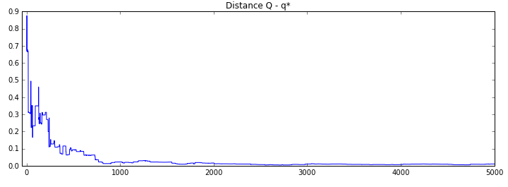
'A': A, 'N' : N, 'R' : R, 'Q' : Q}In this implementation, we also keep track of the state of the agent at every step, and can for example look at how its action value estimates converge towards the actual action values with the increasing number of steps:
The chapter discusses other action selection methods: optimistic initial values selection, upper-confidence-bound selection, and gradient bandits. The code for these methods together with some comparisons between them are available in the IPython notebook that I already mentioned above.